Writing New Image Hashing Algorithms to Help a Yearbook Teacher

A friend of mine came to me with a seemingly innocuous problem. They run the school’s yearbook class, and the students will often accidentally reuse the same photo in different places. A lot of time gets spent throughout the year tediously combing through and looking for these duplicates. Imagine having to memorize and identify all the different photos used throughout a 200 page book! So I agreed to help out and write a program to do the work instead. It seemed easy at first; extract images from a bunch of PDFs and throw some image hashing at the problem. How hard could it be? Oh how wrong I was…

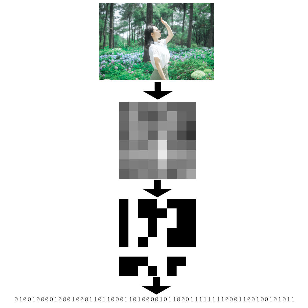
There are many ways to find duplicates images, but the most robust methods involve perceptual hashes. These algorithms “hash” the image in such a way that an image will match even if it has been scaled, cropped, rotated, etc. Average Hash, for example, does this by scaling the input image down to 8x8 and outputting a 1 or a 0 bit for all 64 pixels based on whether that pixel is greater than or less than the average. Changing the image’s resolution, brightness, color, etc won’t affect such a hash much (if at all). For the most part, all perceptual image hashing algorithms work similarly.

Perceptual hashes are simple, powerful algorithms that get used in things like reverse image search engines. Yet they have a certain weakness that made them all unsuitable for the task at hand. The photos used in the yearbook were often heavily cropped and rotated. Consider this example:

In that example there are two images, each cropped from the same source image. They are duplicates, but they would not be detected by existing perceptual hashes because only part of the images match. Popular perceptual hashes also cannot handle large rotations. Even delving into recent perceptual hashing research, the algorithms just aren’t designed to handle extreme cases like these. Luckily reading those research papers inspired an idea for a potential solution.

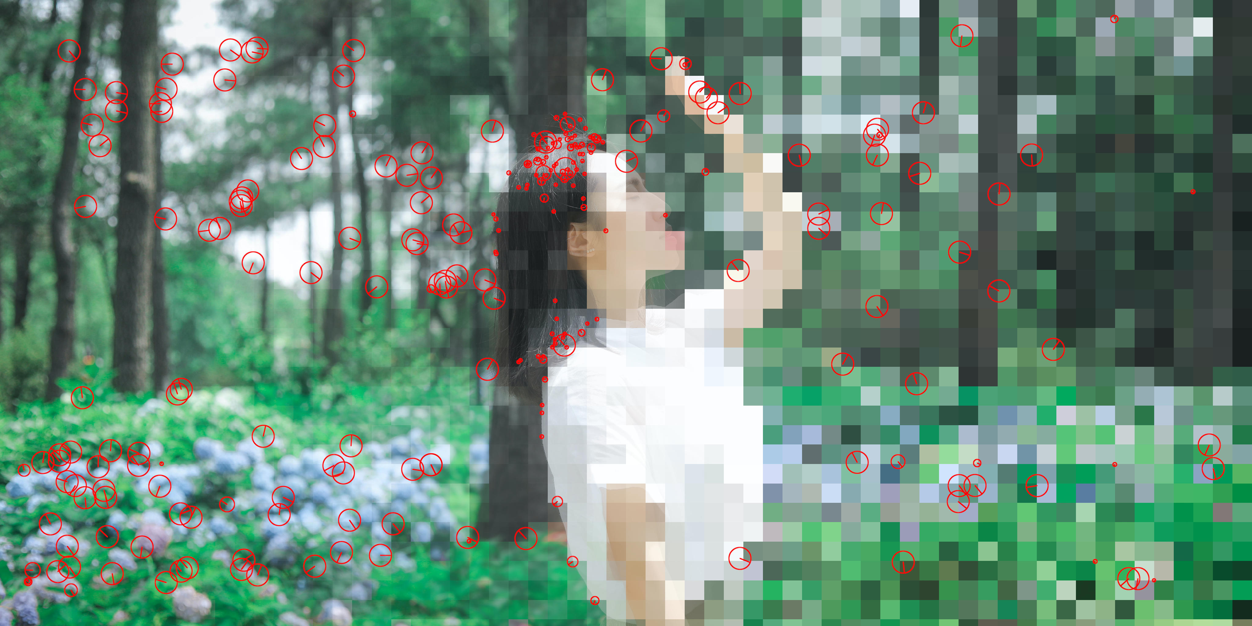
The first and most important piece of the puzzle involves feature extraction. There is a field of computer vision based around extracting salient “features” from an image. Before the dawn of deep neural networks, these feature based algorithms were used for things like object detection. Given an image they spit out a set of landmarks, or “keypoints” as they’re called, in the image, and a “description” (feature vector) for each of those keypoints.

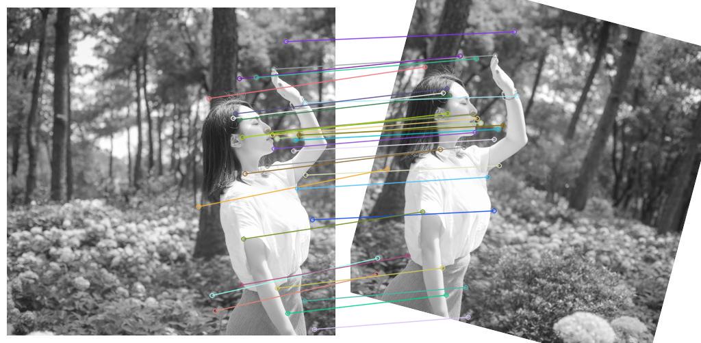
The most important part is that the features these algorithms find are stable under various transformations. You can scale, rotate, translate, and otherwise manipulate the image and the same features would tend to be found. Perfect for our task! Looking again at the cropping example above, we would hope that any features it detects in the matching halves of the images will be exact matches. Perhaps we can find duplicates by looking for any images where at least some of the detected features match.

So now there’s a possible algorithm. Run feature detection to get a set of features for each image. Compare all possible pairs of images. In any given pair, if some amount of their features “match” then they might be a duplicate image. To keep things simple I ignored the locations of the features and only match based on their descriptions. So that gives us two bags of feature vectors that can be brute force compared. With a few experiments I was able to confirm that this algorithm works! When two images weren’t duplicates their features almost never matched up. When they were duplicates, at least a few features were near identical.

It’s true that the location of the features could be important. More correctly, the relative locations of matching features. It’s likely that considering this information would make a better matching algorithm, but it turns out to be good enough without that specificity.

Now I had an algorithm that worked where all other perceptual hashes failed. It wasn’t time for champagne just yet, though. There remained one more difficult challenge: search. These feature detection algorithms can spit out thousands of features per image. And I was working with a set of tens of thousands of images to compare. A naive search would involve searching every combination of every image (with n=10000 that would be 50 million comparisons). Every comparison involves yet another naive search to compare all the features (with just n=1024 features that’s half a million comparisons). That amounts to 25 trillion feature vector comparisons. Yikes.

To make this tractable the search needs to be less naive. There are many different tree and index based approaches that could be used. Locality Sensitive Hashing proved to be the winner. LSH is kind of like a HashMap. With a HashMap if two keys are exactly the same they’ll end up in the same bucket. So HashMaps can be used to quickly find exact matches. LSH can be used to find things that are near matches. Imagine being able to “look up” each feature vector and find other feature vectors that are similar to it. Perfect for our problem.

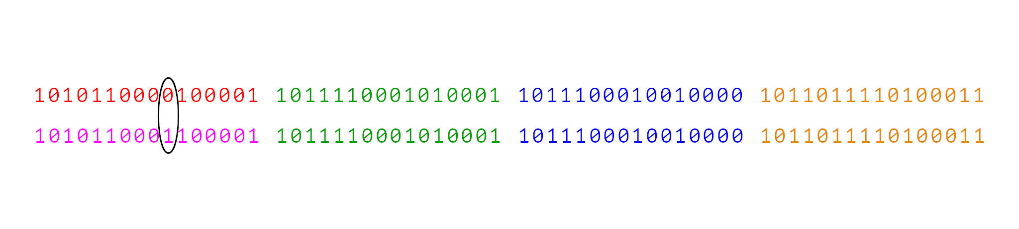
The version of LSH I used is quite clever and worth elucidating. The feature vectors themselves are 512-bit vectors where the similarity between two features is measured by the number of differing bits (the hamming distance). To index these using an LSH, these 512-bit vectors first get permuted (mix the bits up in a predetermined way) and then split into thirty two 16-bit pieces. Those 16-bit pieces are actually 32 different “hashes”, from which we build 32 different indexes. The result of this is that if two features differ by 31 bits or less they are guaranteed to end up in at least one bucket in the index together.

Why? Consider two features that differ by 1 bit. In that case, given the above procedure, it’s clear that those two features will still share 31 hashes. Hence they will end up sharing a bucket together. Similarly if they differ by 2 bits they will share at least 30 hashes. Even if two features differ by 31 bits they will still have at least one hash in common.

With this technique all features could be indexed, and the buckets of those indexes could be searched for matches. Because our distance threshold for matching features is less than 31, this method is guaranteed to find all matches. Most importantly this algorithm runs 100x faster than a naive search!

With this and liberal application of Rust, optimization, and multithreading the program went from spending several days of runtime to a couple minutes. It’s amazing what a little computer science can do, huh?

Those were the hardest pieces of this program. I also spent some time running experiments on a test dataset to pick the best feature extraction algorithm. There are many, but of all the ones in OpenCV, BRISK performed best in this application. The dataset also let me calibrate the permutation used in the LSH hashing, which turned out to be important since the bits in the feature vector are highly correlated. And finally the program has two tunable hyperparameters: Distance Threshold and Score Threshold. Distance Threshold is the threshold used for determining if two feature vectors are “similar”. Score Threshold is used for comparing potentially matching images. A score is calculated by dividing the number of matching features by the total number of features. If it’s greater than the threshold, the images match. By calibrating these hyperparameters the algorithm was tuned such that it caught all but one of the most pathological duplication tests, and let only a rare few false positives through.

The final program had a quick GUI thrown on it for selecting the set of PDFs to be processed, and to view and filter the results. My friend ended up using the app for this year’s yearbook and it performed splendidly. Not only did it catch obvious duplicates, it also caught a few really hard to find duplicates that a human would have likely missed. Nothing like inventing cutting edge computer vision algorithms to fix a school’s yearbook.